How to use
This page walks through the recommended workflow for processing a folder of images with Projection Traces (PT), then describes secondary features and the headless mode.
Workflow at a glance
For algorithmic detail, see How it works.
Step 1 — Open an image or folder
Use File > Select an Image… (Ctrl+I) and pick any TIF/CBF/HDF5 file. PT loads the file, discovers all sibling images in the directory, and shows the image in the Image tab (Fig. 1).
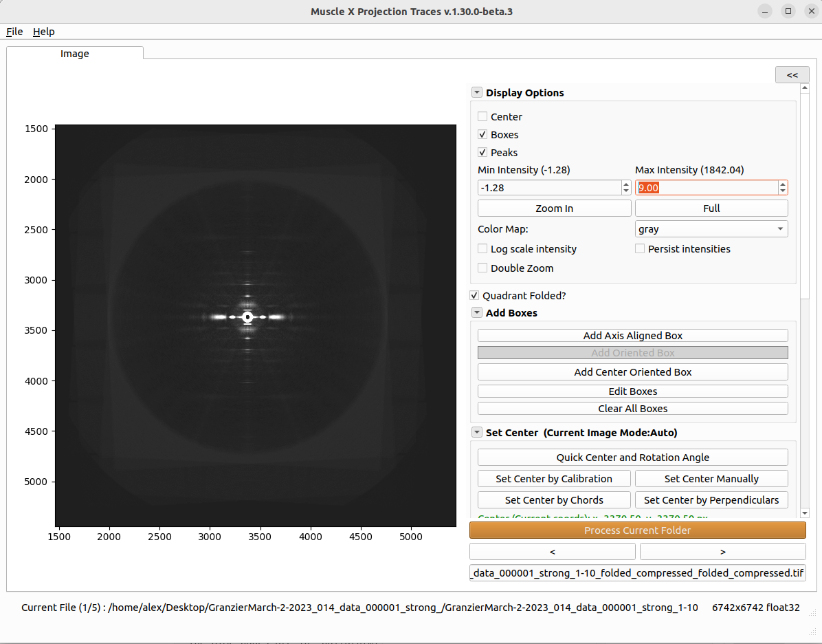
Fig. 1 Projection Traces main window after an image is loaded. The Image tab shows the diffraction pattern; the right panel holds the center/rotation and box controls.
By default PT writes results into the same folder as the input. Use File > Change Output Directory… if the input is read-only or you want results in a separate location.
PT will not produce results yet — you still need at least one box and one peak selection. The remaining steps configure those.
The bottom-bar arrows (< / >) walk image by image; <<< / >>> walk by HDF5 file. Process Current Folder reprocesses every image in the folder with the current boxes and peaks.
Step 2 — Center, rotation, and Quadrant Folded mode
Getting an accurate diffraction center and rotation angle is critical — every box, peak mirror, and projection is computed relative to them, so a center or angle that is even slightly off will bias every result downstream. Set them carefully on the first image; the same values are then propagated to every other image in the folder.
Quadrant Folded checkbox (top of the right panel) — check this if the input is already quadrant-folded. PT will then take the diffraction center to be (width/2, height/2). If unchecked, the center is taken from auto-detection or the manual tools below.
Center group — Quick Center and Rotation Angle, Set Center by Chords, Set Center by Perpendiculars, Set Center by Calibration, Set Center Manually. Use Apply Center to propagate to other images in the folder.
Set Rotation Angle group — Set Auto Orientation (algorithm choice + Mode Orientation), Set Angle Interactively (click two points to define the meridional axis), Set Angle Manually (type the angle).
For full details on these shared tools, see Common Settings — Diffraction Center and Rotation. For calibration, see Common Settings — Calibration Settings.
The Pattern Settings (Optional) group has one PT-specific value:
Mask Threshold — pixels at or below this value are excluded from convex-hull background estimation. Default is −999 (effectively off). Lower this only if your image has invalid pixels that should be ignored during background fitting.
Step 3 — Add and edit boxes
Boxes define the rectangular regions whose contents will be projected to 1-D. After you drag out a box, a detail dialog asks for its name, projection axis, and background-subtraction mode (Fig. 2). The Add Boxes group on the right panel has three buttons:
Button |
Drawing |
Use when |
|---|---|---|
Add Axis Aligned Box |
Drag a corner and release. A dialog asks for a name, the projection axis (horizontal or vertical), and a background-subtraction mode. |
The features you want to integrate run along the equator or the meridian. |
Add Oriented Box |
Currently disabled in the UI. |
— |
Add Centered Oriented Box |
Click to define the long-axis end-point, then the width. The pivot is fixed at the diffraction center. |
The features lie along a layer line at an angle to the equator/meridian. |
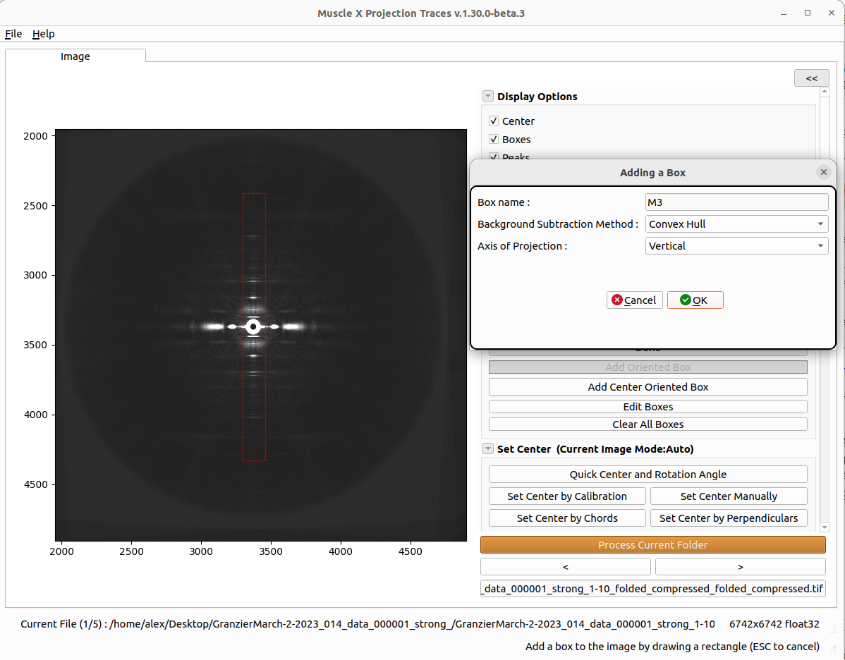
Fig. 2 The box detail dialog that opens after drawing a box: set the name, projection axis, and background-subtraction mode before accepting.
Each box becomes its own tab at the top of the window (Fig. 3). The box’s projection axis is its long axis; the projection is the sum of intensities along the short axis.
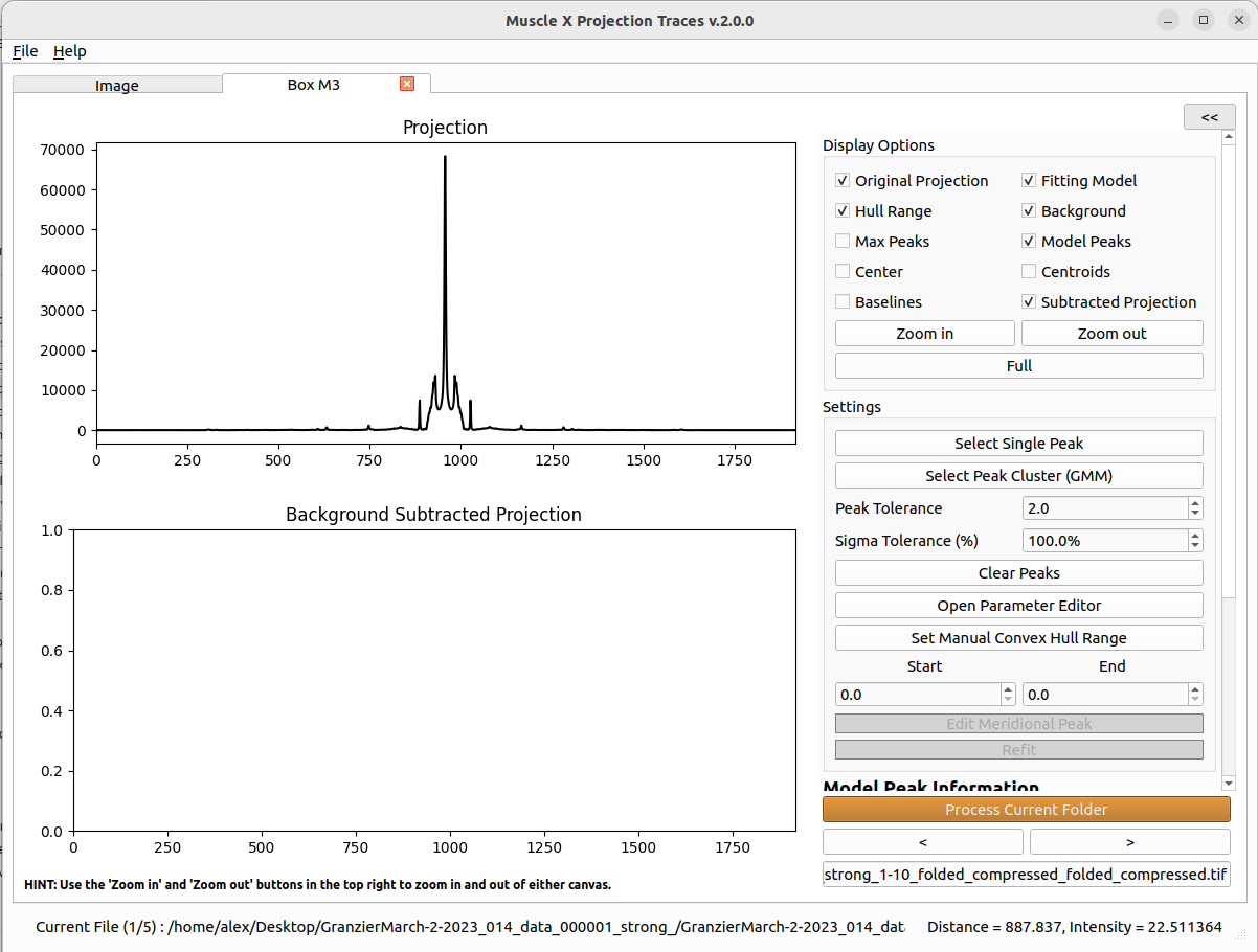
Fig. 3 A box tab. Each box has its own tab with the 1-D projection plot and the per-box background, peak-selection, and fit controls.
When the box detail dialog opens, you choose one of three Background Subtraction modes per box:
Fit model (default) — PT fits a per-peak Gaussian plus up to three central Gaussians (overall background, meridional background, meridional peak) that act as the background.
Convex hull — PT removes a convex-hull background before fitting; the central Gaussians are not used.
None — no background subtraction.
The mode determines which controls show up in the box tab (e.g. the hull range controls only appear for Convex hull boxes; the Meridional Peak checkbox only appears for Fit-model boxes).
Other controls in the Add Boxes group:
Edit Boxes — open a dialog to resize a selected box (separate height/width with center/top/bottom anchoring).
Clear All Boxes — remove every box and its fit results.
Closing a box’s tab also removes that box.
Step 4 — Select hull range (convex-hull boxes only)
For boxes that use Convex hull background subtraction, the hull range determines where the convex hull is computed on the 1-D projection (Fig. 4). PT initializes it automatically from your peak selections ([min(peaks) − 15, max(peaks) + 15]), but you can override it:
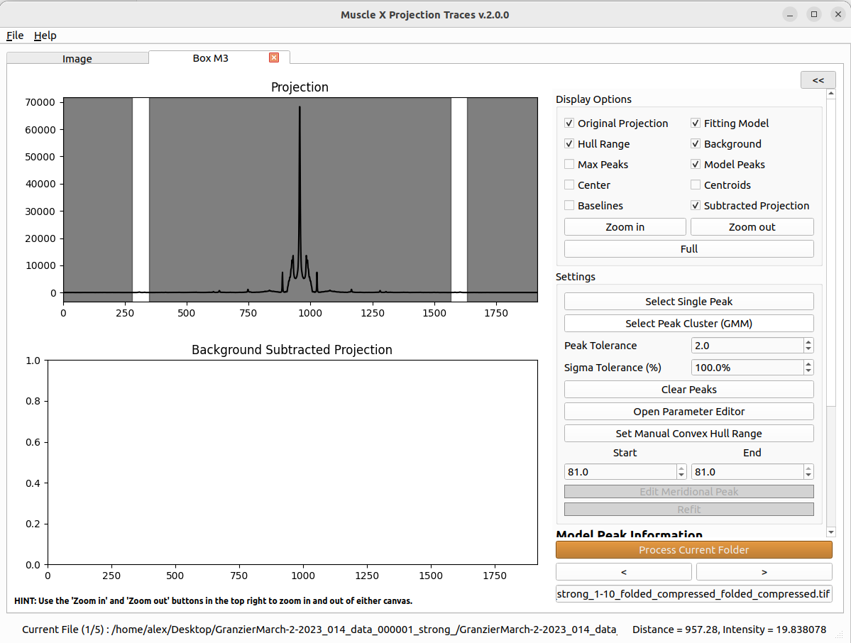
Fig. 4 The convex-hull range marked on the 1-D projection. The hull is computed independently on each half of the projection within this range.
In the box tab, click Set Manual Convex Hull Range and then click two points on the projection plot (start and end). The clicks define the hull range symmetrically about the box center; both halves of the projection use the same range.
Alternatively, type values directly into the Start / End spinboxes in the same group.
The active hull range is also a constraint on where peaks can land during fitting (see Step 5), so it doubles as a way to focus the fit on a specific region of the projection.
Step 5 — Peak selection and fitting
Each box needs at least one peak before fitting can happen. Once peaks are placed and the fit runs, the box tab shows the fitted model over the projection plus the result tables (Fig. 5). There are two paths:
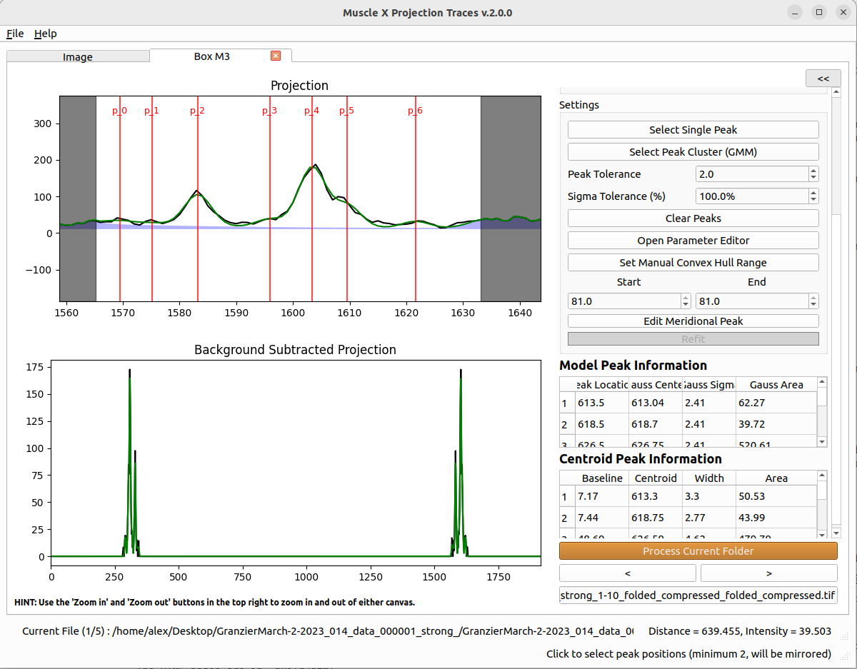
Fig. 5 A box tab after fitting: the projection with the fitted model overlaid (top), the background-subtracted projection with detected peaks (middle), and the Model/Centroid Peak Information tables (right).
Single peak — one Gaussian per peak
In the box tab, click Select Single Peak and click one approximate peak position on the projection plot. PT adds the peak and automatically mirrors it across the box center to create a symmetric pair. Repeat for every reflection you want to fit. Click the button again (or press Done) to exit selection mode.
Each peak gets its own independent Gaussian (independent center, sigma, amplitude).
Fit bounds
Two spinboxes control how tightly the fit is constrained around the seed values:
Peak Tolerance (default 2 pixels) — peak centers can move at most this many pixels from their selected positions.
Sigma Tolerance (%) (default 100%) — initial sigma bounds are
5 × (1 ± tolerance%). Lower this to force narrow peaks; raise it to allow broad peaks.
Per-box options
Meridional Peak checkbox (Fit-model boxes only) — when checked, the fit includes a dedicated narrow Gaussian for the meridional peak; when unchecked, only the wider background Gaussian remains.
Edit Meridional Peak — opens a dialog to fix or constrain the meridional peak’s center, sigma, or amplitude.
Refit — re-runs the fit with the current parameters and constraints (useful after editing Peak/Sigma Tolerance or fixing parameters).
Clear Peaks — removes all peaks and resets the fit.
After fitting, two tables on the right side of the box tab show the results:
Model Peak Information — per peak: Peak Location, Gauss Center, Gauss Sigma, Gauss Area.
Centroid Peak Information — per peak: Baseline, Centroid, Width, Area.
You can edit a peak’s baseline by double-clicking its Baseline cell — this regenerates the centroid, width, and area for that peak from the new baseline.
The plot canvases above the tables show, from top to bottom, the original projection with the fitted model overlaid, and the background-subtracted projection with the detected peaks. The Display Options group lets you toggle every overlay (original projection, fit model, background, hull range, model peaks, max peaks, baselines, centroids, subtracted projection).
Step 6 — Parameter Editor
For complete control over the fit, click Open Parameter Editor in the box tab (Fig. 6). The dialog shows every fit parameter (p_i, sigma_i, amplitude_i, common_sigma in GMM mode) with:
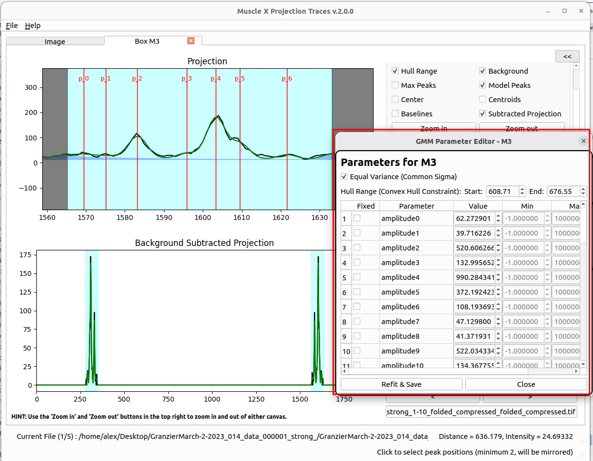
Fig. 6 The Parameter Editor dialog. Each parameter row has Value, Min/Max bounds, and a Fixed checkbox; the top controls toggle Equal Variance (Common Sigma) and the hull range.
Value — current best-fit value (editable).
Min / Max — bounds (editable, persisted per box).
Fixed — checkbox to lock the parameter during refitting (
vary=False).
Additional controls at the top:
Equal Variance (Common Sigma) — toggle GMM mode for this box (forces all peaks to share one sigma, or restores per-peak sigmas).
Hull Range — Start / End — change the convex-hull range live (only enabled for Convex-hull boxes).
Interactive hull range editing on the graph
While the Parameter Editor is open, the hull range is drawn as a highlighted band on both projection plots (top and bottom). You can adjust it directly with the mouse (Fig. 7):
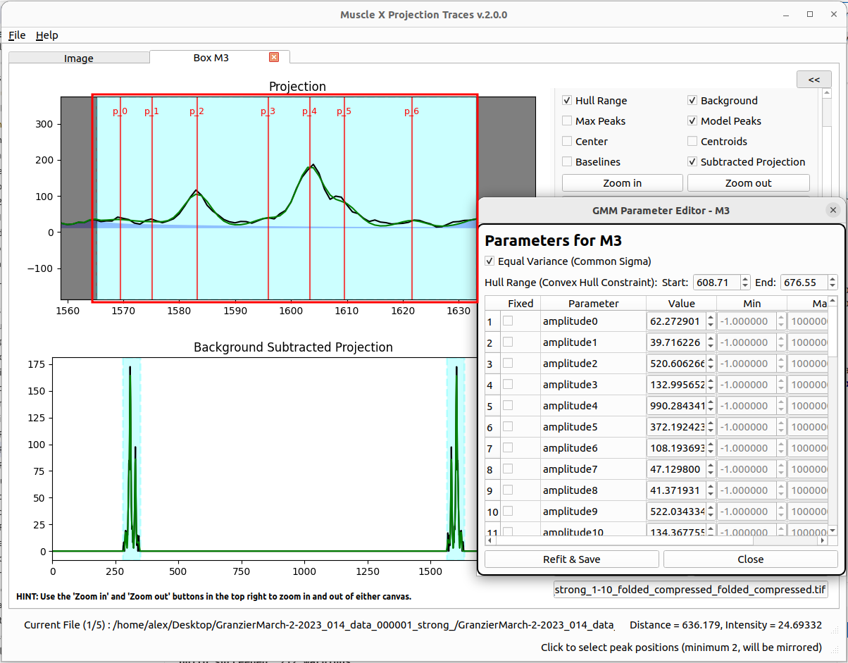
Fig. 7 Interactive hull-range editing. Drag an edge of the highlighted band to move one bound, or drag inside the band to shift the whole region and its peaks together.
Drag an edge (left-outer, left-inner, right-inner, or right-outer boundary of the band) to move only that bound. The opposite side stays put. Hover near an edge and the cursor changes to a horizontal resize arrow.
Drag inside the band (away from any edge) to shift the whole region together with all the peaks by the same offset. Useful when the diffraction pattern has drifted but the relative spacing of the peaks is unchanged.
All drag edits update the Parameter Editor’s spinboxes (Hull Range Start/End) and peak rows in real time, but — like the rest of the dialog — they remain in preview until you click Refit & Save.
The dialog runs in preview mode: edits are reflected on the plot in real time, but they are not committed until you click Refit & Save. Close discards any unsaved edits (already-saved edits from prior Refit & Save are kept).
Typical use cases:
Fix the meridional reflection’s position when you know it shouldn’t move between images.
Tighten the sigma bounds for a poorly resolved peak.
Switch a single box between Single-peak (per-peak sigma) and GMM (common sigma) without leaving the dialog.
Step 7 — Navigate to the next image
Once one image is fully configured (center, rotation, boxes, peaks, optional Parameter Editor edits), PT uses image N’s fit output as image N+1’s input instead of the original user clicks. Navigation and batch processing are driven from the bottom bar (Fig. 8):
> / < — go to the next/previous image and process it immediately.
Process Current Folder — process every image in the folder.
Process Current H5 File / Process All H5 Files — same for HDF5 input.
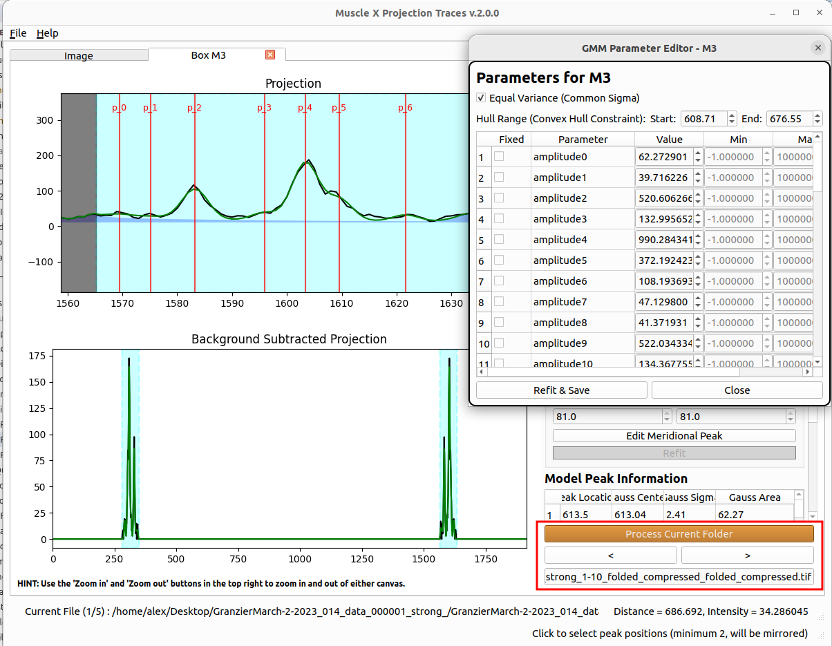
Fig. 8 The bottom navigation bar: single-step arrows (< / >), HDF5 file arrows (<<< / >>>), and the batch-processing buttons.
.. tip:: For batch QA, it's convenient to leave the Parameter Editor open while navigating between images. PT remembers each editor's position and size, automatically closes it on image switch, and reopens it after the new image finishes processing — so the table always shows the current image's freshly-fit parameters in the same place on screen.
What carries forward to the next image
After each successful fit, PT writes the following back into a folder-level template (pt_cache/boxes_config.json):
Refined peak positions — the lmfit-converged centers (
p_i) replace the user-clicked seeds. The next image starts its fit from these refined positions, so peaks track gradual drifts across a series.Box geometry — coordinates and type (axis-aligned / oriented / centered).
Per-box settings — background mode (
bgsub), meridional-peak flag, hull range, GMM mode (use_common_sigma), Peak/Sigma Tolerance.Center, rotation, calibration, mask threshold — global settings.
What does not carry forward
Fit parameter bounds (
param_bounds) — reset to empty for each new image, so per-image Parameter Editor edits (Min/Max/Fixed) do not contaminate later frames.Per-image fit results (sigmas, amplitudes, errors) — re-fit from scratch using the inherited peak positions as initial values.
Rejection flag and comments — these are per-image.
Caching
Per-image cached results from previous sessions are reloaded automatically when revisiting an image; the fit is not re-run unless a setting changes. To force a fresh run, delete the pt_cache folder under the output directory, or use the -d flag in headless mode.
Output files
After processing, PT writes the following under the chosen output directory:
pt_results/summary.csv
One row per image. Columns are auto-generated based on the configured boxes; for each box and each peak the table records both Gaussian fit outputs and centroid-based outputs, in pixels and (when calibration is set) in nm. Representative column names:
FilenameBox <name> Maximum Point <i> right/left (Pixel | nm)Box <name> Gaussian Peak <i> right/left (Pixel | nm)Box <name> Gaussian Sigma <i> right/leftBox <name> Gaussian Area <i> right/leftBox <name> Centroid <i> right/left (Pixel | nm)Box <name> Centroid Area <i> right/leftBox <name> Average Centroid Area <i>— mean of left/right centroid areas.Box <name> Average Gaussian Area <i>— mean of left/right Gaussian areas.Box <name> Background Sigma,Background Amplitude— overall background Gaussian.Box <name> Meridian Background Sigma,Meridian Background Amplitude— meridional background Gaussian.Box <name> Meridian Sigma,Meridian Amplitude— meridional peak Gaussian.Box <name> error— normalized fit residual.Box <name> comments— auto-populated with"High fitting error"whenerror > 0.15, otherwise-.reject—rejectedif the image was rejected (see below), otherwise-.comments— per-image user comments.
pt_results/center_log.csv
One row per image with the diffraction center used (center_x, center_y) and the per-box centerX (the center coordinate translated into each box’s local frame). Useful for spotting outliers in center detection across a batch.
pt_results/1d_projections/ (optional)
Written only when Export All 1-D Projections is checked. For each image and each box, two tab-separated text files are produced:
<name>_box_<box>_original.txt— the raw 1-D projection.<name>_box_<box>_subtracted.txt— the background-subtracted projection.
pt_cache/
Pickled processing state used to skip recomputation when the same image is re-opened with the same settings. Delete this folder (or use -d in headless mode) to force reprocessing.
Other features
Reject image and comments
Each image has a Reject this image checkbox and a Comments editor on the right panel:
Reject this image — sets the
rejectcolumn torejectedfor that file.Comments / Edit / Clear / Submit / Cancel — write a free-text note that ends up in the
commentscolumn.
Useful for flagging frames that failed to process correctly or recording notes about specific measurements during a long batch.
Display options on the Image tab
The top-right of the Image tab has three PT-specific checkboxes: Center, Boxes, Peaks. These toggle the corresponding overlays on the displayed image. All other display controls (intensity range, log scale, colormap, zoom, persistence) are shared with other MuscleX modules.
Save and load settings
File > Save Current Settings (
Ctrl+S) — write the current calibration, boxes, peaks, and per-box parameters toptsettings.json. Use this on a representative configuration and reuse it via headless mode or File > Load Settings (Ctrl+L) in a future session.File > Load Settings — load a settings file.
Headless Mode
For batch processing without a GUI:
musclex pt -h -i <file.tif> [-s ptsettings.json] [-d]
musclex pt -h -f <folder>   [-s ptsettings.json] [-d]
Arguments:
-i <file>— process a single file.-f <folder>— process every image in the folder.-s <settings.json>— load a settings file generated by File > Save Current Settings in the GUI. Without this, PT has no boxes to integrate and will exit without producing results.-d— delete the existingpt_cachebefore processing.
.. note:: On Windows, replace ``musclex`` with ``musclex-main.exe`` (typically under ``C:\Program Files\BioCAT\MuscleX\musclex``).
Multiprocessing on folders
The headless runner processes one image per CPU core. Output for each worker is prefixed with the process index so interleaved log lines can be untangled.
ptsettings.json
The recommended way to produce this file is to configure one image fully in the GUI and use File > Save Current Settings. The exact key names depend on the boxes you have created; inspect a generated file and musclex/modules/ProjectionProcessor.py / musclex/headless/ProjectionTracesh.py if you need to hand-edit values for headless runs.