The Equatorial Diffraction Pattern from Striated Muscle
A good introduction to X-ray diffraction of vertebrate muscle can be found in Chapter 2 of Squire, JM, The Structural Basis of Muscular Contraction, Plenum 1981. A treatment of X-ray diffraction from insect flight muscle can be found in Irving (2006) X-ray Diffraction of Indirect Flight Muscle from Drosophila (in Nature’s Versatile Engine: Insect Flight Muscle Inside and Out, J Vigoreaux editor Landes Biosciences, Georgetown, TX).
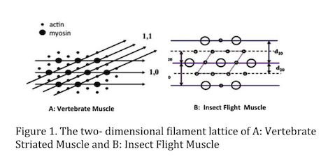
The equatorial pattern arises from the projected density of mass in the A-band of the sarcomere. The thick filaments are packed into a hexagonal lattice with thin filaments interdigitated between them either in the trigonal positions (vertebrate muscle - Figure 1A) or half way between adjacent thin filaments (many insect flight muscles - Figure 1B). The density of the filaments projected onto a plane therefore represents a two dimensional crystal with the hexagonal lattice points occupied by thick filaments. One can draw imaginary planes through the crystallographic unit cell (see Figure 1A for vertebrate muscle) corresponding to various values of the so-called Miller indices h & k. In figure 1A are drawn the lattice planes corresponding to the h=1, k=0 (separated by d10) and h=1, k=1 separated by d11). These lattice planes give rise to the two strongest pairs of X-ray reflections in the X-ray diffraction pattern, the 1,0 and 1,1 reflections respectively with intensities I1,0 and I1,1. In insect muscle, the two strongest pairs of reflections are the 1,0 and 2,0 reflections because of its different lattice geometry (Figure 1B).
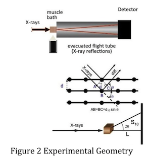
Figure 2 shows the geometry of a muscle diffraction experiment. The muscle sample is separated from the detector by a distance L. The spacing between thick filaments is ~ 40 nm, large compared to the wavelength of X-rays (~0.1nm). Bragg’s Law, n λ = 2dsinθ, describes the relationship between the lattice spacing d and the scattering angle 2θ. If d is large, θ will be small. L therefore is typically 2-3 m so that the distance S10, the distance from the center of the pattern to the 1,0 reflection, is of the order of a few mm. The scattering angle, 2θ, can be calculated from tan -1 (S10/L). At small angles however, tan2θ ≅ sin2θ ≅ 2θ. Substitution into Bragg’s law and solving for d10 gives a simplified expression: d10= nλL/S
It should be clear from this analysis that the lattice spacing is inversely proportional to S10. In skinned cardiac muscle the 1,1 and 1,0 equatorial reflections are often the only reflections visible. In skeletal muscle additional diffraction peaks past the 1,1 are frequently visible corresponding to other, higher order diffraction planes in the crystallographic unit cell denoted by larger values of h and k. In vertebrate muscle the first 5 such equatorial reflections are the 1,0; 1,1; 2,0; 2,1 and 3,0. In insect flight muscle, one can observe as many as 20 equatorial reflections. In addition, in skeletal muscle there is a peak located between the 1,0 and 1,1 reflections coming from the insertion of the thin filaments into the Z-band and is called the Z-band reflection. The position of this reflection from the center of the pattern is about 1.46 x S10 (Yu et al., 1977 J. Mol. Biol. 115:455-464). In general, the positions of the A-band reflections, excluding the Z-band reflection, obey a hexagonal lattice selection rule where S(h,k) = sqrt( h2+k2+h*k)*S10. Thus, d10 may be calculated from any equatorial reflection and applying the hexagonal selection rule. The d10 lattice spacing can be converted to inter-thick filament spacing by multiplying d10 by 2/√3).
The intensities of the 1,0 and 1,1 equatorial reflections may be determined from one-dimensional projections along the equator. When cross bridges bind to the thin filaments in vertebrate muscle there are radial and azimuthal movements of the crossbridges so there is a loss of mass on the 1,0 planes (containing only thick filaments) and a gain of mass on the 1,1 planes (Huxley, H. E. 1968. J. Mol. Biol. 37:507-520. and Haselgrove, J. C., and H. E. Huxley. 1973. J. Mol. Biol. 77:549-568). As a consequence, the intensities of the 1,0 reflections decreases and the 1,1 increases. I11/I10 intensity ratios, therefore, can be used to estimate shifts of mass from the region of the thick filament to region of the thin filament. Graded levels of isometric force
There is additional information in the equatorial patterns in the form of the widths of the diffraction peaks. It has been shown, Yu et al., 1985 Biophys J 47 :311-321, that the width of the Gaussian or Voigtian functions used to approximate the shape a given peak σh,k may be expressed (Yu et al., 1985 Biophys J 47 :311-321, Irving & Millman 1989) J Muscle Res Cell Motil. 10:385-94) as √(σc2+σd2Shk2+σs2Shk2), where Shk=√(h2+k2+hk)*S10 as above. σc is the known width of the X-ray beam, σd is related to amount of heterogeneity in inter-filament spacing among the myofibrils, and σs is related to the amount of paracrystalline (liquid-like) disorder of the myofilaments in the hexagonal lattice. Liquid-like disorder is sometimes called disorder of the second kind (Vainshtein, B. K. 1966. Diffraction of X-rays by Chain Molecules.Elsevier, Amsterdam.). σd can be expressed relative to Δd10/d10 as a measure of the width of the distribution of lattice spacings between the different myofibrils in the sample. σs can be expressed in terms of ΔX/d10 where ΔX is the standard deviation in the distribution of distances between nearest-neighbor unit cells in a given myofibril. σs increases substantially during contraction in skeletal muscle (Yu et al., 1985 op. cit.). Because of the dependency of the peak width on the square of the scattering angle, liquid like disorder rapidly causes the peaks to become indistinguishable from the background at higher scattering angles. The muscle lattice can also exhibit disorder of the first kind (Vainstein, 1966 op. cit.) which is the tendency of objects to vibrate isotropically around the lattice positions due to thermal energy resulting in a linear decrease in diffracted intensities with increasing scattering angle. This is often called “temperature factor type disorder” in crystallography. There is no direct way to estimate the degree of this kind of disorder without invoking a model structure.