How to use
After launching Equator, select an image file or a failedcases.txt file with File > Select a File (or Failed Cases)… (Ctrl+O). Equator displays the image and processes it with the current settings. If valid cached results already exist for the current program version and preprocessing settings, the cached results are loaded instead of being recalculated.
File and output options
Use File > Process Current Folder (Ctrl+F) or the Process Current Folder button to process all images in the current folder. For HDF5 input, use Process Current H5 File to process all frames in the selected HDF5 file.
Use File > Change Output Directory… if results, cache files, and failed-case lists should be written somewhere other than the input data directory. This is useful when the raw data directory is read-only or when you want to keep analysis output separate from the source images.
Use File > Clear All Caches in Current Folder (Ctrl+D) to remove existing Equator cache files from the selected output directory and force images to be processed again.
Use File > Save Current Settings (Ctrl+S) to export the current Equator processing and fitting settings to eqsettings.json. Calibration, blank image, and mask settings are not stored in this JSON file; they are managed by the shared workspace settings. Use File > Load Settings… (Ctrl+L) to load a saved Equator settings file and reprocess the current image.
Image tab
The Image tab shows the processed image and overlays. Display options let you adjust intensity limits, log scaling, colormap, zoom, and overlay visibility for center, R-min, R-max, histogram, integrated area, and detected peaks. Fitting Error Threshold (shown in the display options area) sets the maximum acceptable normalized fit error; images whose fit exceeds this threshold are flagged in the results. Display options do not modify the raw image data.
For shared center, rotation, calibration, restore/apply, and Double Zoom tools, see Common Settings — Diffraction Center and Rotation.
For empty cell subtraction and mask configuration, see Common Settings — Empty Cell Image and Mask. Equator-specific mask behavior is described in Empty Cell Image and Mask.
The Image Processing panel contains Equator-specific controls:
Set R-min and Set R-max define the radial range used for the equatorial analysis. You can also use Fixed R-min and Fixed R-max to reuse explicit pixel values that persist across images.
Set Box Width defines the integration area used to build the equatorial projection histogram. Use Fixed Box Width to keep the same integration height across images.
Find Orientation with Brightest Spots and Orientation Finding control the method used for automatic rotation/orientation detection.
Mask Threshold sets the value below which pixels are treated as invalid (masked) during Equator processing. The default is −0.01.
Inpainting fills invalid or masked pixels before processing. Use this cautiously; it is mainly for visualization and gap handling, not for changing raw quantitative measurements.
Rotate 90 rotates the result by 90 degrees. Persist Rotation keeps that rotation setting when navigating to subsequent images.
Reject marks the current image as rejected. Rejected images are recorded in the summary output and failed-case list.
Reset All clears all manually set processing parameters (R-min, R-max, box width, rotation) and returns Equator to fully automatic detection for the current image.
Fitting tab
The Fitting tab shows the projection histogram, convex-hull-subtracted curve, detected peaks, and fitted model. Use the display checkboxes to show or hide the original histogram, convex hull result, fitting graph, peaks, Z line, and center X marker.
General fitting settings
Number of peaks on each side — minimum is 2. Equator fits this many equatorial reflections on each side of the center.
Model — choose Gaussian or Voigt. The Voigt model adds a gamma (Lorentzian fraction) parameter per side. If only I11 and I10 are visible (4 reflections total), the Voigt model is over-determined; fix sigma S or gamma on each side to resolve this.
Skeletal Muscle (Z line) — adds a Z-line peak to the fit (for skeletal muscle patterns). Enables the Z-line fixed-parameter controls in each side panel.
Extra Peak — adds an additional free peak to the fit. Enables the extra-peak fixed-parameter controls in each side panel.
Start Manual Peak Selection — use when the automatically detected peaks need correction. Click peaks on the histogram and press Done.
Left and right fitting panels
Each side (left and right) has its own panel with the following controls. These settings apply independently to the two halves of the equatorial pattern.
Main peak parameters (Settings group)
Control |
Description |
|---|---|
Fixed Sigma C |
Fix σC (crystallite size broadening) to the entered value. When unchecked, σC is a free parameter. |
Fixed Sigma D |
Fix σD (disorder broadening) to the entered value. When unchecked, σD is a free parameter. |
Fixed Sigma S |
Fix σS (sampling broadening / sigma S) to the entered value. Useful for constraining poorly-determined patterns. |
Fixed Gamma |
Fix the Lorentzian fraction γ (Voigt model only). When the model is Gaussian, this control is hidden. |
Z-line parameters (Skeletal Muscle group — enabled when Skeletal Muscle is checked)
Control |
Description |
|---|---|
Fixed Center |
Fix the Z-line peak position (in pixels from center). |
Fixed Intensity |
Fix the Z-line peak amplitude. |
Fixed Sigma |
Fix the Z-line peak width (σ). |
Fixed Gamma |
Fix the Z-line peak shape (γ, Voigt model only). |
Extra peak parameters (Extra Peak group — enabled when Extra Peak is checked)
The extra peak has the same four fixed-parameter controls as the Z-line group (Fixed Center, Fixed Intensity, Fixed Sigma, Fixed Gamma), applied to the additional free peak.
Global fitting options
Fixed Background K — when checked, fixes the background slope constant K to the entered value (default 0). When unchecked, K is a free parameter in the background model. Fixing K at 0 forces a flat background; freeing it allows a linear background under the peaks.
Use Previous Fit — initializes the current image’s fit from the previous image’s fitted parameters. Useful for time-series data where conditions change slowly.
Refit current image — re-runs the fitting pipeline with the current settings without reprocessing the image from scratch.
Refit current folder — applies the current fitting configuration to every image in the folder.
Results and parameter editing
The Results tab summarizes the current image’s fitting output, including peak areas, S10, d10 when calibration is available, I11/I10, fitting error, and related model parameters (σD, σS, γ).
The Parameter Editor tab exposes the current lmfit parameter set for advanced manual refitting. You can directly edit parameter values, bounds, and whether each parameter is fixed or free. These edits are intended for the current refit session; use File > Save Current Settings to persist fitting settings across sessions.
Output files
Equator writes results to an eq_results folder under the selected output directory. If no separate output directory is selected, eq_results is created inside the folder containing the selected image.
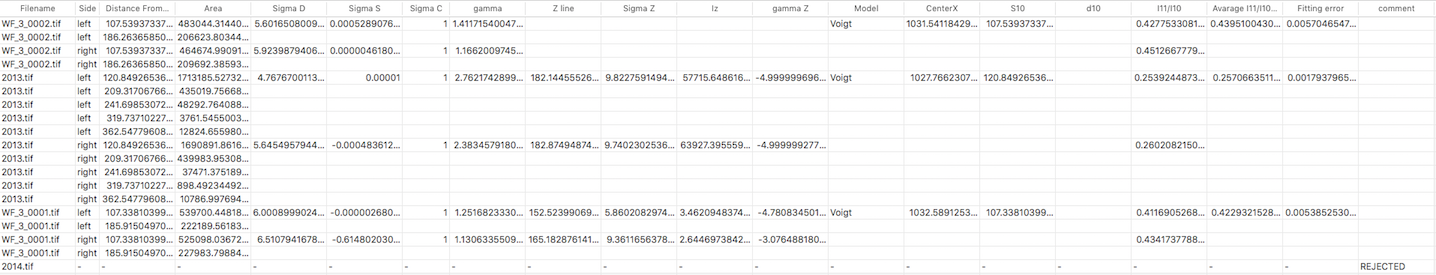
summary.csv — one row per reflection peak per image. Multiple rows are written for a single image when more than one peak is fitted.
summary2.csv — the same results in a transposed layout: one row per image, with all peak values for that image laid out as columns. This format is more convenient for spreadsheet analysis.
failedcases.txt — a list of images that could not be processed automatically. An image is added to this list when it has no effective peaks, the model fitting fails, the fitting error exceeds the threshold, or the image is manually rejected. You can reload this file with File > Select a File (or Failed Cases)… to step through and manually fix each case.