Common Settings
Several configuration settings and image-processing algorithms are shared across multiple MuscleX modules. Rather than repeating them in each module’s documentation, they are described here once.
Modules that use these settings: Quadrant Folding (qf), Equator (eq), Projection Traces (pt), Add Intensities Single/Multiple Experiment (aise/aime), and X-Ray Viewer (xv, center tools only).
Table of Contents
Calibration Settings
A calibration image is a diffraction pattern from a calibrant with a ring at a known d-spacing. By fitting this ring to a circle, MuscleX can refine the diffraction center and use the fitted radius to convert distances in pixels to reciprocal-space values. The same dialog also accepts calibration geometry directly and can reuse a previously saved calibration.info file.
Implementation Details
The calibration circle is fitted numerically to a set of user-selected or automatically detected points on the calibrant ring. The fitting minimises the residuals between the selected points and a geometric circle model. When advanced optimisation is enabled, a Differential Evolution global search is used to escape local minima, followed by MAD-based outlier rejection (Median Absolute Deviation statistics) to discard poorly placed points, and a multi-start refinement to select the best result from several initial guesses.
The fitted radius and Calibrant ring d-spacing determine the calibration scale. When wavelength λ and pixel size are available, MuscleX can infer the sample-to-detector distance (SDD). Parameter-based calibration uses λ, SDD, and pixel size directly. The dialog displays the computed scale and inferred SDD beneath the parameter fields. From this geometry, MuscleX computes d10 using Bragg’s law:
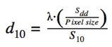
Fig. 14 d10 formula relating wavelength, sample-to-detector distance, S10, and pixel size.
How to Use
Set by Calibration Image
Open Set Center by Calibration, check Enable Setting by Calibration Image, and use Browse to select a calibration image.
Inspect the fitted circle — the center and radius are overlaid on the image if the ring is found automatically (see Fig. 15).
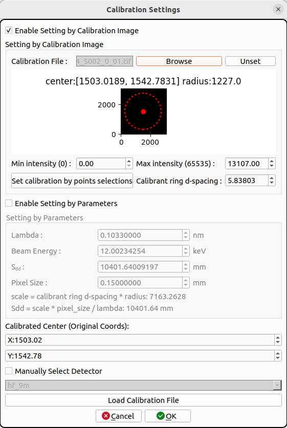
Fig. 15 Calibration dialog showing the automatically fitted circle overlaid on a calibrant ring image.
If the fit is wrong or missing, click Set calibration by point selections to open the Manual Calibration Dialog (see Fig. 16).
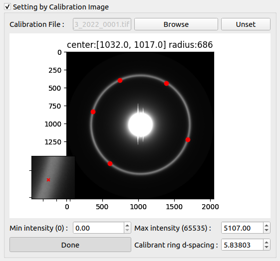
Fig. 16 Manual Calibration Dialog showing the main image (left) and zoom view (right) for precise point selection.
Select points on the ring using the two-step process: click once on the main image for the approximate location, then click in the zoom view for the precise location. Select at least 5 points, ideally 8–12 spread evenly around the ring.
Enter the calibrant ring d-spacing and click Done, then OK. The image is reprocessed with the new calibration.
When an image is loaded, MuscleX first checks FabIO detector/header metadata and then compares the image shape with detectors in the pyFAI registry. If a detector is identified, its pixel size is filled automatically. Header pixel-size fields are used as a fallback. The detected source is saved with the calibration so it can be reviewed when the calibration is reused.
Load a Saved Calibration
Click Load Calibration File and select a saved
calibration.infofile.MuscleX restores its image- or parameter-based calibration values, detector metadata, pixel-size source, and calibrated center.
Review the restored values and click OK. If the original calibration image is missing, the saved numeric values are still loaded and a warning is shown.
Use this workflow to apply an established calibration without repeating the ring selection. The imported calibration remains separate from a reusable application settings JSON file.
Set by Parameters
Check Enable Setting by Parameters.
Enter either Lambda (nm) or Beam Energy (keV). The two values remain synchronized using the standard energy–wavelength conversion.
Enter Sdd (mm) and Pixel Size (mm), or use an automatically detected detector pixel size. These values are used directly to calculate the reciprocal-space scale (see Fig. 14), bypassing ring fitting.
Review the computed scale and SDD readouts, then click OK.
Pixel size now begins as Unknown instead of assuming a detector value. If it cannot be identified from the detector or image header, MuscleX asks for it when you accept a parameter calibration. Cancelling that prompt leaves the Calibration Settings dialog open without saving incomplete geometry.
Calibrated Center
The Calibrated Center (Original Coords) fields show the center that will be returned to the calling application. They are populated by the fitted calibration circle or by a loaded calibration. For parameter calibration, review or edit the original-image X and Y coordinates before accepting. If the input is already quadrant-folded, the center is fixed at the geometric center and these fields are read-only.
Manually Select Detector
Normally, leave Manually Select Detector unchecked so MuscleX can use FabIO metadata and pyFAI shape matching.
Check it to override automatic detection, then choose a detector from the sorted pyFAI registry. The list also includes
MAR_165_2x2for 2×2-binned MAR 165 images.Editing Pixel Size manually clears the manual detector association so the saved calibration does not claim detector-derived geometry that no longer matches the entered value.
Diffraction Center and Rotation
The diffraction center is the point of zero scattering vector — where the direct beam hits the detector. The rotation angle aligns the equatorial axis of the diffraction pattern with the horizontal axis used by the processing algorithms.
Implementation Details
Finding the Diffraction Center
To find the center automatically, the image is first converted to 8-bit and a Gaussian filter is applied to reduce noise. Thresholding is then applied, and the center is estimated by fitting an ellipse to the largest contour of the thresholded image (see Fig. 17 and Fig. 18).
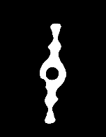
Fig. 17 Thresholded diffraction image. The largest contour is used to estimate the diffraction center.
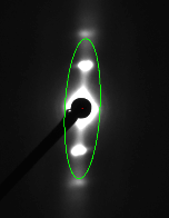
Fig. 18 Diffraction image after automatic center detection. The detected center is marked on the pattern.
If the fitted center is at a fractional pixel position, the image is translated so that the center falls on the nearest integer coordinate. If no ellipse can be fitted, the center is computed using the moments method from OpenCV.
Calculating the Rotation Angle
The program first estimates a rotation angle by fitting an ellipse to the diffraction pattern. It then refines the angle using pyFAI’s azimuthal integrator in two passes: an initial pass over 360 values (one per degree) to locate the highest-intensity peak, followed by a second pass at 0.1-degree resolution around that peak for precision (see Fig. 19). If the refined angle is close to the ellipse-fit estimate, the refined value is used; otherwise the ellipse estimate is returned. The angle returned is always the closest acute angle.
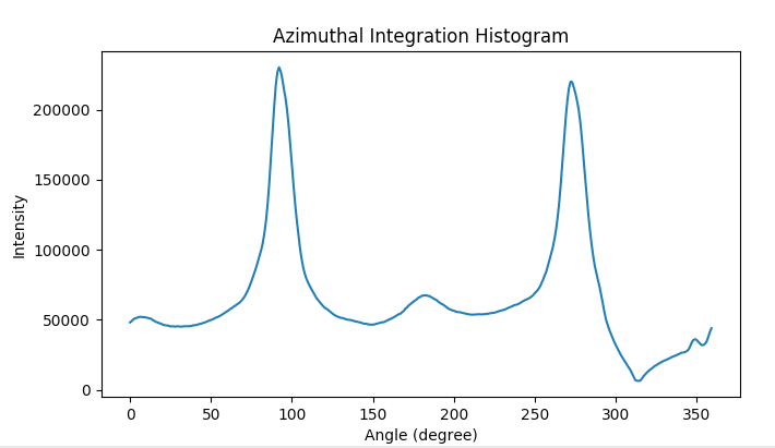
Fig. 19 Azimuthal integration histogram. The dominant peak identifies the rotation angle of the diffraction pattern.
How to Use
All center and rotation tools can be combined with Double Zoom for sub-pixel accuracy.
Quick Center and Rotation Angle
Zoom in to the region of the diffraction pattern for easier placement.
Click Quick Center and Rotation Angle.
Click the first reflection peak on one side of the equator.
Click the corresponding opposite peak on the other side of the equator. The center and rotation are computed from the midpoint and angle of the two clicks (see Fig. 20).
Press ESC to cancel.
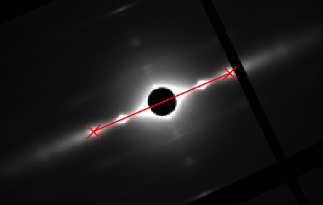
Fig. 20 Quick Center and Rotation Angle tool. Two opposite reflection peaks are selected; the program derives the center and rotation from their midpoint and connecting angle.
Center and Rotation Mode Indicators: The interface shows whether automatic or manual center/rotation is active.
Set Center By Chords
Zoom in to the diffraction region.
Click Set Center By Chords.
Click multiple points along the circumference of the diffraction ring. Perpendicular bisectors (blue lines) appear as you select points (see Fig. 21).
Click the button again when done. The center is the average of the perpendicular bisector intersections.
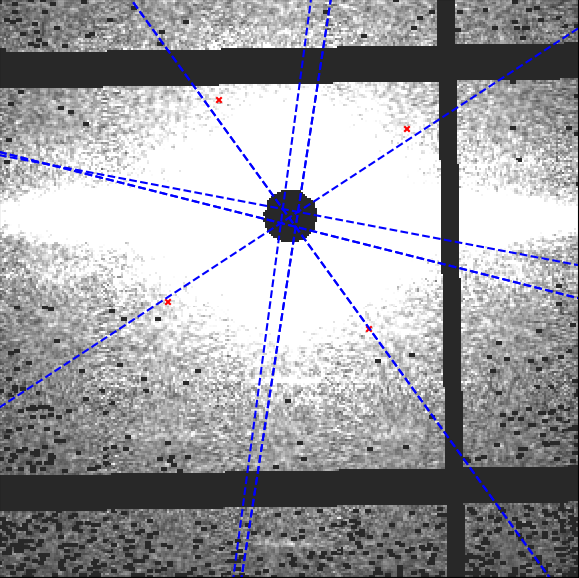
Fig. 21 Set Center By Chords. Blue perpendicular bisectors to the chords intersect near the diffraction center.
Set Center By Perpendiculars
Zoom in to the diffraction region.
Click Set Center By Perpendiculars.
Click pairs of reflection peaks: first a peak on one side of the equator, then its opposite on the other side (horizontal pair). Repeat for vertical pairs (above/below equator). Each pair defines a line through the center (see Fig. 22).
Click the button again when done. The center is the average of all line intersections.
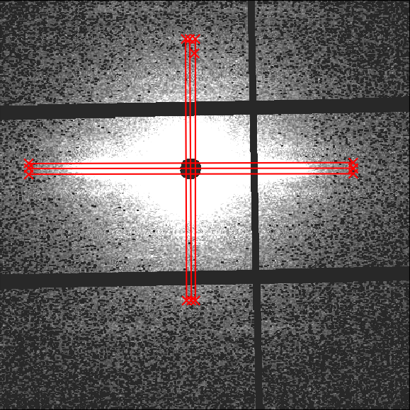
Fig. 22 Set Center By Perpendiculars. Pairs of opposite peaks define horizontal and vertical lines whose intersections locate the center.
Set Rotation Angle
Click Set Rotation Angle (assumes the center is already correctly placed).
Move the line until it aligns with the equatorial axis of the diffraction pattern (see Fig. 23).
Click to accept the rotation angle. Press ESC to cancel.
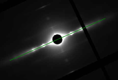
Fig. 23 Set Rotation Angle tool. The interactive line is dragged to align with the equatorial axis.
Refine Center and Rotation
Use refinement after an automatic or manually estimated center and rotation are already close:
Click Refine Center. The refinement runs registration, gradient, and local-search stages and may take a few minutes.
In the confirmation dialog, enable Also refine rotation if both refined values should be saved. Otherwise, only the refined center is applied.
Click Refine Rotation to search for a better angle while keeping the current center fixed.
Review the old and new values in the result message. Accepted results are stored as manual center/rotation settings and the current image is reprocessed.
Refinement quality depends on a useful starting estimate and a pattern with sufficient symmetry. It is intended to improve an existing solution, not replace initial center and orientation detection.
Double Zoom
Double Zoom provides sub-pixel accuracy when placing center or rotation control points. A 20×20 pixel region around the cursor is cropped and scaled up 10× in a subplot (see Fig. 24).
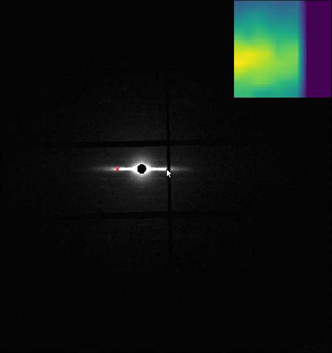
Fig. 24 Double Zoom panel (top right). The 20×20 pixel region around the cursor is shown at 10× magnification for sub-pixel point placement.
Check the Double Zoom checkbox — the subplot appears.
Click a calibration button (e.g. Quick Center and Rotation Angle).
Move the mouse to the approximate position and click to freeze the subplot.
Click the exact location in the subplot — the corresponding point is placed on the main image.
Repeat for the second point.
Uncheck Double Zoom to hide the subplot.
Restoring Automatic Settings
Click Restore Auto Center to remove manual center values. Choose the current image, subsequent images, previous images, or all images.
Click Restore Auto Rotation to remove manual rotation values using the same scope choices.
Use Apply Center or Apply Rotation to copy the current value to subsequent, previous, or all images. In QF, selecting multiple batch folders extends the all images scope across that selected batch.
Center and Rotation Management
Configuration Fingerprinting: When center or rotation settings change, the result cache is automatically invalidated to keep results consistent.
Manual Settings Preservation: Manual center and rotation values are preserved during cache operations.
Per-folder Persistence: Manual geometry is written immediately to the authoritative settings area for each source folder, including previous/subsequent/all propagation across a selected QF batch.
Alignment Snapshots: QF alignment detection captures the saved geometry once at the start of a detection pass. Edits made while the dialog remains open appear in the table the next time detection starts, keeping each pass internally consistent.
R-min
R-min is the minimum radius from the diffraction center that is included in the analysis. Pixels closer to the center than R-min — typically dominated by the beamstop shadow — are excluded from histogram projection, peak fitting, and all downstream calculations.
Implementation Details
The program builds a radial intensity histogram (x-axis: radius in pixels, y-axis: summed intensity). R-min is set to the radius at which the histogram first falls to 50% of its maximum value (see Fig. 25). To prevent over-removal, this radius is constrained to be no more than 150% of the radius of the maximum. For example, if the maximum is at radius 35, R-min is searched in the range 36–59 (35 × 1.5 ≈ 53, but the hard limit is 59 = 35 × 1.5 rounded up with a small margin). If the 50% threshold is not found within this range, R-min defaults to the upper bound.
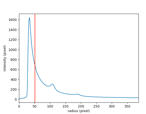
Fig. 25 Radial intensity histogram used to determine R-min. The dashed line marks the 50% maximum threshold; R-min is set at the crossing point.
Herman Orientation Factor
The Herman Orientation Factor (HoF) quantifies the degree of orientational order in the diffraction pattern. It is used by Scanning Diffraction and related modules.
Implementation Details
After azimuthal integration produces a circular intensity histogram (see Fig. 19), the Herman Orientation Factor is calculated for each degree using:
x is either 180° or 90°, yielding one HoF value per degree in the histogram. See Page 7 of this reference for properties of the Herman Factor.
The figures below show the HoF concept and representative results from integration over 90° and 180°.
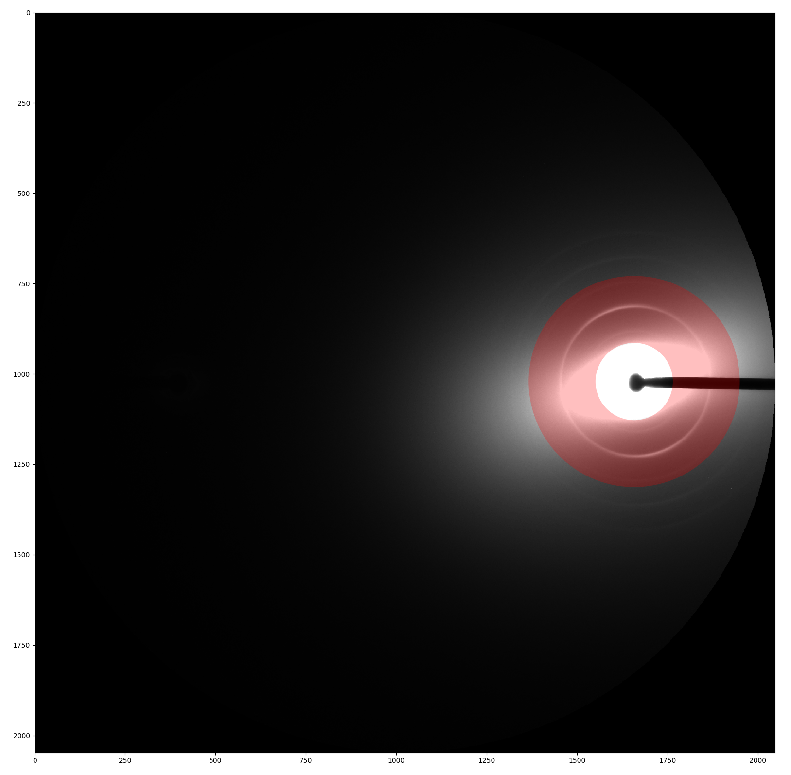
Fig. 26 Schematic of the azimuthal angle φ used in the Herman Orientation Factor formula.
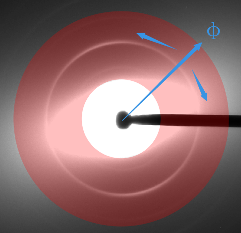
Fig. 27 Azimuthal intensity histogram with the Herman Orientation Factor integration illustrated.
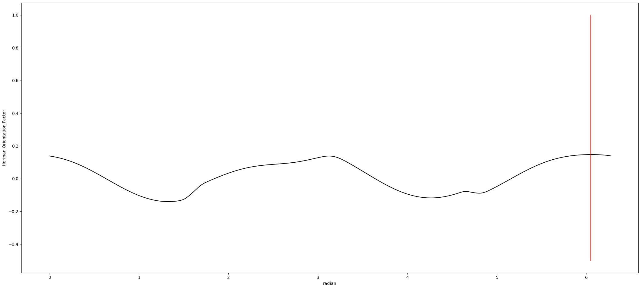
Fig. 28 Herman Orientation Factor results from azimuthal integration over 90°.
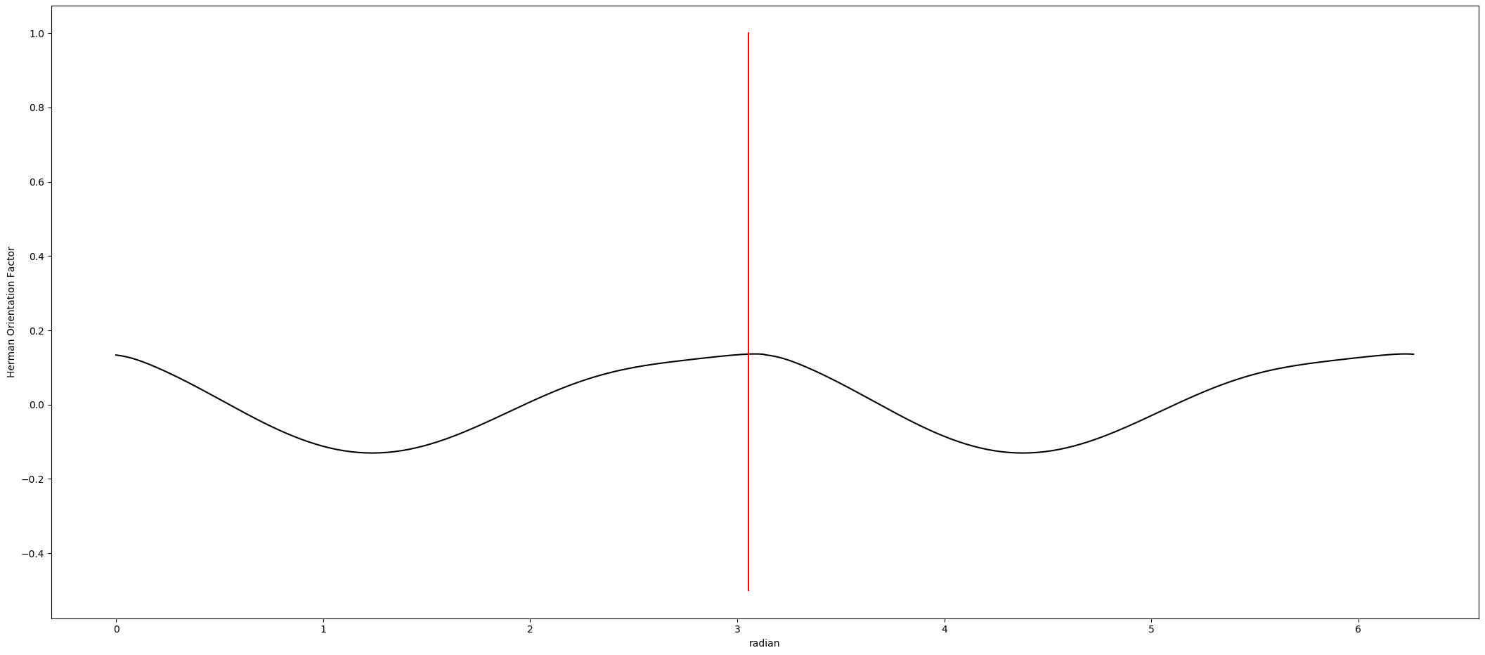
Fig. 29 Herman Orientation Factor results from azimuthal integration over 180°.
Empty Cell Image and Mask
These two independent settings — Empty Cell Image and Mask — are configured through the Apply Empty Cell Image and Mask panel in the processing workspace. Each has its own button to open its dialog, and each can be independently enabled or disabled via a checkbox once its settings have been saved.
Implementation Details
Empty Cell Subtraction
A diffraction pattern from a muscle sample is the sum of the true muscle signal and a background contribution from the sample holder, solvent, and beam path. Subtracting an empty cell image — a pattern recorded without a sample — isolates the muscle diffraction signal, which is important for accurate peak fitting and intensity ratios.
When Apply Empty Cell Image is checked, the program scales the empty cell image by the configured scale factor and subtracts it from the working image before any analysis. Pixel values that become slightly negative after subtraction (due to noise) are clipped to zero.
Masking
A mask is a binary image marking which pixels should be ignored during processing. When Apply Mask is checked, the program loads mask.tif before analysis begins. Each pixel where mask == 0 is overwritten with a sentinel value of −1.0 in the working array. The raw file on disk is never modified. If empty cell subtraction is also enabled, it runs first; the mask sentinel assignment follows.
Masked pixels are excluded from histogram projection, peak fitting, and all downstream calculations. In modules such as Equator, ignored columns are interpolated over to preserve a continuous diffraction profile for fitting. See each module’s documentation for details on how masking interacts with its specific analysis pipeline.
How to Use
Empty Cell Image
Click Set Empty Cell Image in the processing workspace panel to open the Empty Cell Subtraction dialog.
Click Select Empty Cell Image to browse and select a single empty cell image file (any format supported by
fabio, e.g..tif,.edf,.cbf). A status indicator turns green when the image is loaded.Adjust the Empty Cell Image Scale spin box (range 0–1000, default 1.0) to match the empty cell exposure to the sample exposure. The difference image updates live as you change the scale.
Compare the images using the radio buttons:
Option
Description
Difference Image (Original − Empty Cell)
Shows the subtraction result at the current scale. This is the image that will be processed.
Original Image
Shows the raw sample image with no subtraction.
Empty Cell Image
Shows the empty cell image scaled by the current factor.
Click Save. The configuration is written to
blank_image_settings.jsonin the settings folder, and the Apply Empty Cell Image checkbox in the main panel becomes enabled. Uncheck it at any time to temporarily disable subtraction without deleting the configuration.
When you reopen the same image directory, the saved empty cell image path and scale factor are loaded automatically, and the checkbox is restored to its last saved state.
Mask
Click Set Mask in the processing workspace panel to open the Set Image Mask dialog.
Configure one or more mask methods in the Mask Options group. Their combined result is previewed as a color overlay in real time:
Drawn Mask
Click Draw Mask to launch the
pyFAI-drawmasktool. Paint arbitrary regions using geometric tools (polygon, rectangle, brush, etc.).After closing the tool, the mask is loaded automatically. Enable the Drawn Mask checkbox to include it.
Drawn regions are shown as a red overlay.
Low Mask Threshold
Enable the Low Mask Threshold checkbox to mask all pixels below the specified value (default −0.01). This targets detector gaps or dead pixels assigned a negative sentinel value.
Optionally enable Enable Mask Dilation with a 3×3, 5×5, or 7×7 kernel to expand the low-threshold mask outward — useful for border pixels adjacent to sensor gaps.
Low-threshold regions are shown as a green overlay.
High Mask Threshold
Enable the High Mask Threshold checkbox to mask all pixels above the specified value (default 64,000). This targets saturated pixels on 16-bit detectors.
The same optional dilation controls are available.
High-threshold regions are shown as a blue overlay.
Review the color legend:
Color
Meaning
Green
Low Mask Threshold
Blue
High Mask Threshold
Red
Drawn Mask
Purple
Rmin / Rmax mask (applied by the main processing window)
Click Save. The following files are written to the settings folder:
mask_config.json— threshold values and dilation kernel sizes.drawn-mask.edf— the rawpyFAI-drawmaskoutput (if a drawn mask was created).mask.tif— the final combined binary mask applied during processing.
If all three methods are disabled when you click Save, all mask files are removed and the mask is cleared entirely. The Apply Mask checkbox in the main panel becomes enabled once
mask.tifexists. Uncheck it to temporarily disable the mask without deleting the saved settings.
When you reopen the same image directory, the saved mask configuration is loaded automatically and the checkbox is restored to its last saved state.