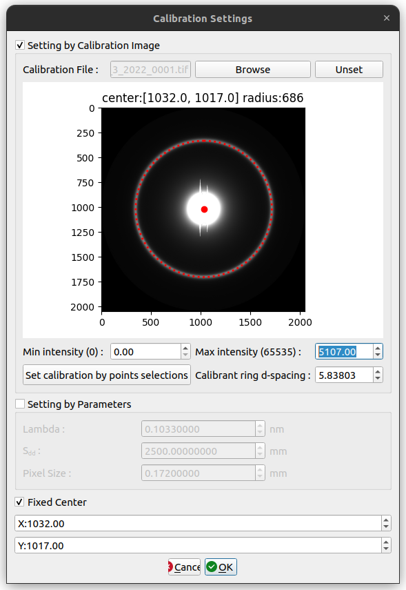
Calibration Settings
A calibration image is a shot of a membrane sample that gives a ring in the diffraction pattern at a known spacing in inverse nm. By fitting this ring to a circle you can refine a center and you can use the radius of the ring to convert spacings in pixels to spacings in nm.
Setting by Calibration Image
When the box is selected, you can choose a calibration image and the program will try to fit a circle to the image. The center and radius will be shown on it if the circle can be fitted.
However, if the circle cannot be fitted or the circle is in the wrong position, you can also fit the circle manually by clicking on “Set manual calibration by point selections” button. Once the button clicked, you will see another image at the bottom left which is the zoom area of your cursor. To select a point on the ring, you need to click a first time on the image (approximate click), then a second time on the zoom area (precise click).
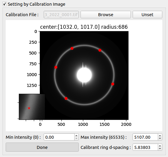
You will have to click at least 5 points on the ring position, and click Done when you finish. After setting appropriate calibrant ring d-spacing, and clicking OK, the image will be reprocessed with new calibration settings including center and d-spacing.
Advanced Manual Calibration
.. note:: **New in version 1.27.0**: The manual calibration dialog now includes advanced optimization methods for improved accuracy and robustness.
When you click “Set manual calibration by point selections”, the Manual Calibration Dialog opens with several advanced features:
Point Selection and Refinement
Two-Step Selection Process:
First click: Approximate location on the main image
Second click: Precise location on the zoomed view (bottom left)
This two-step process ensures sub-pixel accuracy
Point Refinement: After selecting a point, the program automatically refines its position by:
Analyzing the local intensity gradient
Finding the exact peak or edge location
Adjusting the point to the optimal position
Visual Feedback: Selected points are displayed on both the main image and zoom view with clear markers
Optimization Methods
The manual calibration uses sophisticated optimization algorithms to fit the best circle through your selected points:
Differential Evolution (Global Optimization):
Escapes local minima to find the globally optimal solution
Uses a population-based search strategy
Configurable population size (default: larger populations for better results)
Multiple generations to refine the solution
MAD-Based Outlier Rejection:
MAD = Median Absolute Deviation
Automatically identifies and removes outlier points
Makes the fit robust against accidentally misplaced points
Uses statistical thresholds to determine outliers
Multi-Start Optimization:
Runs optimization from multiple initial guesses
Selects the best result across all starts
Increases confidence in the final solution
Calibration Dialog Features
Results Display:
Center Coordinates: Shows the refined center position (x, y)
Radius: Displays the fitted circle radius in pixels
Residuals: Shows the fitting error for each point
Optimization History: Track the convergence of the fitting algorithm
Export Options:
Export to CSV: Save the optimization history for analysis
Includes all iterations and parameter values
Useful for troubleshooting or research purposes
Interactive Adjustments:
Add More Points: Continue adding points to improve the fit
Remove Points: Click on a point marker to remove it
Refit: Run the optimization again with current points
Reset: Clear all points and start over
Tips for Best Results
Point Distribution: Select points evenly around the entire ring for best accuracy
Number of Points: Use at least 5 points, but 8-12 points typically give excellent results
Ring Quality: Choose points on clear, well-defined parts of the ring
Zoom Level: Adjust the zoom level to see the ring edge clearly before selecting points
Outlier Handling: Don’t worry too much about one or two imperfect points - the MAD-based rejection will handle them
Understanding the Optimization
The optimization process works by:
Initial Guess: Estimates a rough circle from your selected points
Refinement: Uses differential evolution to find the optimal center and radius
Outlier Detection: Identifies points that don’t fit well (using MAD statistics)
Re-optimization: Refits without outliers for the final result
Validation: Checks that the solution is physically reasonable
The algorithm minimizes the sum of squared distances from each point to the fitted circle, while being robust to outliers.
Troubleshooting
If the fit looks wrong:
Check that you selected points on the actual calibration ring
Try adding more points around different parts of the ring
Remove any obviously misplaced points
Ensure the zoom view was used for precise clicking
If optimization fails:
Make sure you have at least 5 points selected
Check that points are reasonably distributed around the ring
Try clicking “Refit” to run the optimization again
Verify the calibration image has a clear, visible ring
Setting by Parameters
You can also manually set the calibration parameters which are λ, Sdd and Pixel size.
These parameters are used to calculate d10 by 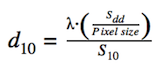
Fixed Center
The center can also be fixed independently of the calibration image. The fixed center checked indicates that the specified center will be used when we move to the next image or process the current folder.
Manually Select Detector
Having a detector corresponding to the images used might improve the results obtained with MuscleX.
You can manually select the detector used for the experiment. If you don’t the detector will be selected automatically by using the size of the image. The list provided is from the pyFAI’s Detectors registry (some name might be repetitive but they point to the same detector). However, if the detector you selected does not correspond to the image provided, the program will fall back to our default detector.