How it works

When an image is selected, Equator applies any configured calibration, center/rotation, empty cell image, and mask settings, then runs the processing pipeline described below. If the image has already been processed with the same MuscleX version and the same preprocessing settings, Equator loads cached results from eq_cache and skips recalculation.

Before Equator-specific processing begins, the shared workspace resolves the diffraction center and rotation angle from automatic detection, calibration, manual overrides, or cached settings. See Common Settings — Diffraction Center and Rotation for details.

Processing pipeline

Equator processes the image in the following steps:

1. Calculate R-min

R-min is calculated using the shared algorithm. See Common Settings — R-min for details.

2. Calculate Box Width

The working image is rotated using the resolved rotation angle, and the area inside R-min is removed. If R-max is set, the area outside R-max is also removed. During rotation the image is expanded as needed so it is not cropped; both square and non-square images are handled.

The box width is initially set to R-min × 1.5. To refine this, the program computes a horizontal histogram of the rotated image, fits a convex hull to estimate the background, and selects the integrated area as the span between the start and end points of the histogram.

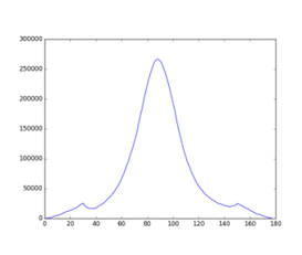
3. Get Intensity Histogram

With the integrated area determined, the program produces a 1-D intensity histogram by summing columns of the rotated image within that area. If a blank image and mask are configured, the original image is subtracted by the blank image before rotation.

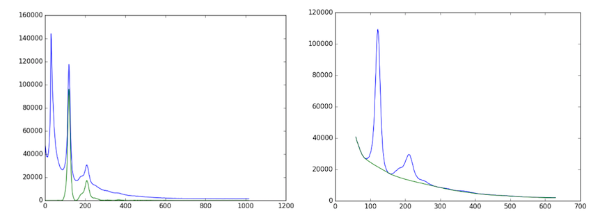
4. Apply Convex Hull to Intensity Histogram

The histogram is split into left and right halves. A convex hull background is estimated independently for each half, using R-min as the starting point, and subtracted to yield a background-free pattern.

During histogram production, columns with values below the mask threshold are treated as ignored. Masked detector gaps are protected during convex-hull background estimation and interpolated before fitting. See Mask and empty cell treatment below for details.

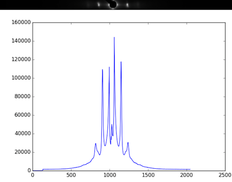
5. Find Diffraction Peaks

Local maxima are located in both the left and right background-subtracted histograms. All candidate peak positions are recorded. Noisy images may produce more candidates than true diffraction peaks; these are filtered in the next step.

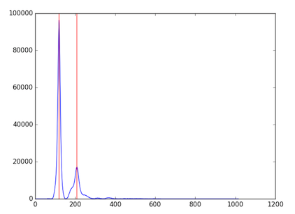
6. Manage Diffraction Peaks

The candidate peak list is validated and corrected before fitting. False positives (peaks from noise) and false negatives (missed reflections) are resolved by searching for the first pair of symmetric peaks to establish S₁₀ — the center-to-first-peak distance on the equator. All remaining peak positions are then calculated from S₁₀ and the lattice angles θ(h,k). The user specifies how many peaks per side to fit (default and minimum is 2).

7. Fit Model

The background-subtracted histogram is fit using the selected model (Gaussian or Voigtian) with initial parameters derived from S₁₀ and the integrated reflection areas. The fit returns the area of each peak, S₁₀, σ_D, σ_S, γ, and I₁₁/I₁₀.

When only 4 reflections are visible (I₁₁ and I₁₀ on each side), the Voigt model is overdetermined. In this case, σ_S or γ should be fixed to avoid degenerate fits.

Mask and empty cell treatment

For information on configuring the empty cell image and mask dialog (selecting an image, scale factor, threshold masking, drawn mask, saving), see Common Settings — Empty Cell Image and Mask.

Stage 1 — Preprocessing (pixel values)

When Apply Mask is checked, the program loads mask.tif before any analysis begins. In this binary image, 0 means “masked” and 1 means “keep”. Every pixel where mask == 0 is overwritten with a sentinel value of −1.0 in the working image array. The raw file on disk is never modified.

If empty cell subtraction is also enabled, it is applied first; the mask sentinel assignment happens afterward.

After blank subtraction, pixel values that become slightly negative (e.g. due to noise) are clipped to 0 before the mask is applied. Sentinel −1.0 therefore remains distinguishable from any legitimate near-zero intensity.

Stage 2 — Analysis (histogram and fitting)

The equatorial analysis works on a column projection histogram: for each x-column of the image, the pixel intensities within the integration area (box height) are summed to produce one value. Masked columns — those containing at least one pixel with a value ≤ −0.01 — are flagged as ignored and handled as follows:

Projection histogram — ignored columns contribute their actual (sentinel-containing) sum but are excluded from the convex hull background estimation. The convex hull algorithm receives an ignore array and uses it to prevent the background baseline from dipping into the artificial gap created by the −1.0 sentinels.
Peak fitting — values in ignored columns within the active hull range are replaced by linear interpolation between the nearest non-ignored neighbors on each side, so the fitted curve is continuous across the gap rather than forced to zero.
Integration area trimming — rows at the top or bottom of the integration box whose entire row sum is ≤ −0.01 are also excluded before the projection is computed.

The net result is that detector gaps, dead pixels, and any other manually masked regions are cleanly bypassed without biasing the background estimate or creating spurious dips in the diffraction profile.

Convex-hull interpolation detail

The processing order is:

Build the raw projection histogram from the integration area.
Detect ignored columns from the rotated working image. A column is ignored if any pixel in that column within the active integration area is at or below the mask threshold.
Run convex-hull background subtraction with the ignore array. During background estimation, ignored columns are lifted out of the way so the baseline does not follow artificial valleys caused by detector gaps or mask sentinels.
After convex-hull subtraction, fill ignored output samples by linear interpolation between the nearest non-ignored neighbors on the already background-subtracted curve.

This interpolation is applied only inside the active hull range (R-min to R-max). Values outside that range remain zero-padded.

This behavior is intentionally scoped to Equator. The shared convexHull() helper retains its original default behavior for other modules. Equator passes convexHull(ignore=...) to protect the background estimate, then repairs the ignored samples in the returned background-subtracted profile so peak fitting sees a continuous curve instead of a hard zero cut.

Optional: Inpainting

If inpainting is enabled (a separate option in the processing panel), masked pixels are filled by the pyFAI inpainting algorithm before the analysis runs. Inpainting estimates each sentinel pixel’s value by interpolating from surrounding valid pixels. This can be useful for narrow gaps where projection-based interpolation is insufficient.

Partial re-runs on manual parameter changes

When a parameter is changed manually, the pipeline does not restart from step 1. Instead, it resumes from the first step that depends on the changed parameter. For example, if Box Width is set manually, the pipeline re-runs from step 3 (Get Intensity Histogram) onward, since the center, rotation angle, and R-min are unaffected.